HOG + SVM

View our interactive Python notebook at Kaggle here.

For this method, we used the Histogram of Oriented Gradients (HOG) approach to extract the features from our images. These features are then classified using SVM. We followed loosely the experiments in Sugiharto and Harjoko (2016) as well as Sugiharto, Harjoko, and Suharto (2020) for this method.

We used HOG from scikit-image and SVM from scikit-learn for this experiment.

Data preprocessing#

We mainly used the Indonesia Traffic Sign dataset from Kaggle. This dataset has 21 classes of traffic signs, but no negative class (images without traffic signs), so we used 100 images from the Road Vehicle Images Dataset from Kaggle as well.

In total, there are 100 images each from the 22 classes as follows:

 1null
 2larangan-belok-kanan
 3petunjuk-area-parkir
 4larangan-masuk-bagi-kendaraan-bermotor-dan-tidak-bermotor
 5perintah-masuk-jalur-kiri
 6perintah-pilihan-memasuki-salah-satu-jalur
 7peringatan-penegasan-rambu-tambahan
 8larangan-berjalan-terus-wajib-berhenti-sesaat
 9lampu-kuning
10larangan-memutar-balik
11larangan-belok-kiri
12peringatan-simpang-tiga-sisi-kiri
13petunjuk-penyeberangan-pejalan-kaki
14lampu-hijau
15peringatan-alat-pemberi-isyarat-lalu-lintas
16larangan-parkir
17peringatan-banyak-pejalan-kaki-menggunakan-zebra-cross
18peringatan-pintu-perlintasan-kereta-api
19larangan-berhenti
20lampu-merah
21petunjuk-lokasi-putar-balik
22petunjuk-lokasi-pemberhentian-bus

We split the dataset with a ratio of train : test = 80 : 20 with stratification. The train data will then be used for k-fold cross validation, so it will later be split again into train and validation. In total, there are 1760 and 440 images for training and testing respectively.

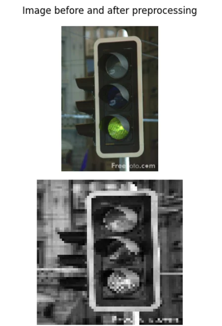
We resized all the images to 128 × 128 in accordance to the papers.

We then performed some traditional preprocessing methods on the images:

• Converting the images to grayscale
• Histogram equalization with CLAHE
• Gamma correction

A comparison before and after preprocessing is as follows.

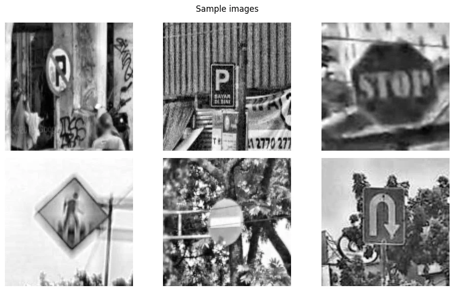
Some sample images after the preprocessing is as follows.

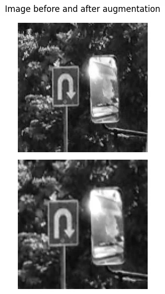
Finally, we prepare a data augmentation function which we will call on our training data (during the k-fold cross validation). This augmentation includes:

• Random rotation by a small angle.
• Random crop and resize.
• Random brightness and contrast adjustment.

A comparison of the original image and the image after augmentation is as follows.

Creating the feature extractor and classifier#

We used Optuna to tune the hyperparameters:

• HOG hyperparameters: Number of orientations, pixels per cell, cells per block, block norm.
• SVM hyperparameters: C, kernel, and gamma.

We ran a total of 50 trials and saved the best models. For each trial, we performed k-fold cross validation with 5 splits, and used accuracy as a metric of selecting the best hyperparameter configuration.

Finally, we did further fine-tuning on the hyperparameters by hand to improve them, trying out small increments in various variables and evaluating the outcome. We managed to achieve a slight improvement in accuracy.

We saved the model outputs to files, which are available to download here.

Evaluating the classifier#

The best hyperparameter configuration is as follows:

1{
2  'orientations': 9,
3  'pixels_per_cell': 13,
4  'cells_per_block': 4,
5  'block_norm': 'L1',
6  'C': 2.5,
7  'kernel': 'rbf',
8  'gamma': 0.0002
9}

We ran the best classifier on the test data. The accuracy is 50.9091%. We plot the confusion matrix as follows.

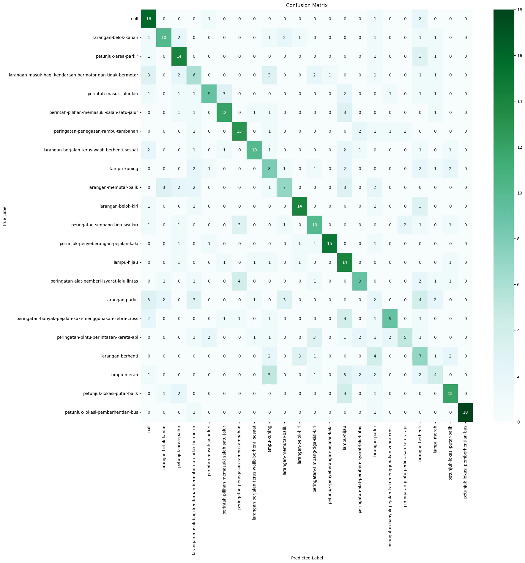
We tried various ways to attempt to increase the performance of the model (changing image sizes, adding more images through augmentation, etc.), but we cannot seem to get the accuracy higher than around 50%. We conjecture that HOG + SVM is not powerful enough to deal with a large number of classes (22) with limited data.

Implementing the sliding window approach#

We followed the papers by implementing overlapping windows (size equal to image size and a step of 16). We then plot the heatmaps for each class separately, calculate the contours, remove overlapping contours, and plot the results on the image. Some sample results are as follows.

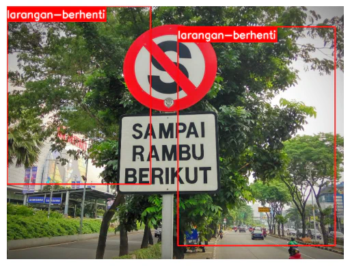
For the first example, it managed to classify the traffic sign, but failed to enclose it completely and instead split the bounding box into two.

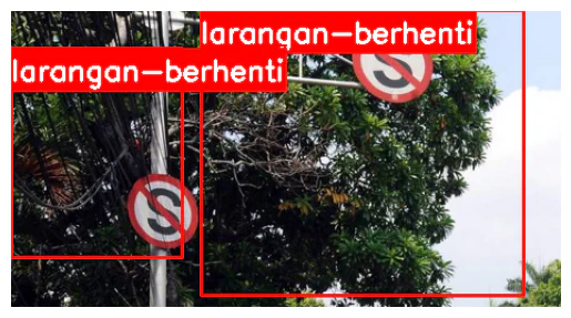
It performed better on the second example: correctly identifying the type of the traffic sign and enclosed both traffic signs entirely.

References#

Sugiharto, A., & Harjoko, A. (2016). Traffic sign detection based on HOG and PHOG using binary SVM and k-NN. 2016 3rd International Conference on Information Technology, Computer, and Electrical Engineering (ICITACEE), 317–321. https://doi.org/10.1109/ICITACEE.2016.7892463

Sugiharto, A., Harjoko, A., & Suharto, S. (2020). Indonesian traffic sign detection based on Haar-PHOG features and SVM classification. International Journal on Smart Sensing and Intelligent Systems, 13(1), 1–15. https://doi.org/10.21307/ijssis-2020-026